Section 1.5 Printing Julia Sets to a Command-Line Interface
May 20th, 2022
Julia sets. Have you heard of those?
If you type 'Julia set' into Google and take a gander at the images, you'll be met with a series of intricate fractals, with spirals and loops every which way.
But what exactly are these weird patterns? How are they generated? And how can we generate them ourselves?
These questions form the core of what we'll be exploring in today's blog post. Join me, as we make a brief jaunt into the world of complex numbers!
Subsection 1.5.1 Keeping it Real
Julia sets live in the world of complex numbers, and frankly, bringing \(i\) into the mix can get confusing. So for now, we'll handle strictly real numbers.
Consider the function \(f: \mathbb{R} \rightarrow \mathbb{R}\) given by
where \(c \in \mathbb{R}\text{.}\) In order to understand what's going on with Julia sets, we're going to examine what happens to the sequence
for certain choices of \(x_0\) and \(c\text{.}\) We're essentially looking at what happens as we keep composing \(f\) with itself.
To get a more concrete idea of this sequence's behavior, we can evaluate some terms for a certain \(x_0\) and \(c\text{,}\) say \(x_0 = 2\) and \(c = -1\text{.}\)
It appears that under these conditions, the sequence grows without bound, so we can say \(A_n \rightarrow \infty\) as \(n \rightarrow \infty\text{.}\) What if we keep \(c = -1\text{,}\) but try a different value of \(x_0\text{,}\) like \(x_0 = 1\text{?}\)
We seem to have entered a loop, where the terms of the sequence periodically alternate between \(0\) and \(-1\text{.}\) In this case, although \(A_n\) doesn't approach anything as \(n \rightarrow \infty\text{,}\) we can be sure that it doesn't blow up to infinity.
This is, in fact, a dichotomy. For any choice of \(x_0\) and \(c\text{,}\) one and only one of the following can be true:
As \(n \rightarrow \infty\text{,}\) the sequence \(A_n\) blows up to infinity, or
It doesn't.
This raises an interesting question. Given a defined value of \(c\text{,}\) can we determine which values of \(x_0\) will cause the sequence \(A_n\) to tend to infinity?
It turns out that we can find a bound \(R > 0\) dependent on \(c\text{,}\) such that if any term of the sequence \(A_n\) satisfies \(|a_n| > R\text{,}\) then \(A_n \rightarrow \infty\) as \(n \rightarrow \infty\text{.}\)
To find a potential expression for \(R\text{,}\) let's consider one property which would be satisfied in the long term if the sequence \(A_n\) tended to infinity. The property in question is
At sufficiently large \(n\text{,}\) this is equivalent to saying that successive terms of the sequence move further and further away from the origin, a behavior which this infinity-approaching sequence would exhibit.
If you, the reader, happen to be an expert in analysis, then I will readily admit that this logic is not quite watertight. For example, a bounded, monotonically increasing sequence would satisfy the inequality, but would not tend to infinity.
However, considering the way the sequence \(A_n\) is defined, we informally expect that such a scenario won't occur. In any case, please forgive my lack of rigor—I am but a measly university undergraduate!
Let's manipulate the inequality \(|a_{n+1}| > |a_n|\) a bit, using the definition of \(f\text{.}\) Suppose \(a_n = x\text{.}\) Then \(a_{n+1} = f(x)\text{,}\) and we perform the following operations.
The third line makes use of the triangle inequality, \(|a| + |b| \geq |a + b|\text{.}\) We now have a quadratic in \(|x|\) on the left hand side, whose roots are
This last expression is our desired value of \(R\text{.}\) To reiterate, if at any point in the sequence \(A_n\) we encounter a term \(a_n\) such that \(|a_n| > R = \frac{1 + \sqrt{1 + 4|c|}}{2}\text{,}\) then \(A_n \rightarrow \infty\) as \(n \rightarrow \infty\text{.}\)
What I've shown here is far from a complete proof, but it hopefully shows, from an informal perspective, how we might have been motivated to find a potential expression for \(R\text{.}\)
Subsection 1.5.2 It's All Complex Now
It's almost time to discuss Julia sets! We've been discussing \(f(x) = x^2 + c\) for so long that it's almost hard to remember what all this talk was in service of.
Before we do that, though, let's bring our function \(f\) into the complex world. We're dealing with a different—but similar—beast this time.
Now consider the function \(f: \mathbb{C} \rightarrow \mathbb{C}\) given by
where \(c \in \mathbb{C}\text{.}\) The filled-in Julia set of \(f\text{,}\) written as \(K(f)\text{,}\) is defined as (set notation warning)
where \(a_n\) refers to the terms of
similar as to before. Now that we're in complex land, though, remember that the absolute value notation refers instead to a complex number's modulus.
The Julia set itself, \(J(f)\) is the boundary of the filled-in Julia set. In notation, it looks like \(J(f) = \partial K(f)\text{.}\) Sidebar: the symbol \(\partial\) means 'boundary'. The boundary of a set in the complex plane has a rigorous meaning, but for our purposes, just think of it like the border, or the perimeter.
The rest of this article is devoted to writing a program that prompts the user for a value of \(c\) and prints the corresponding filled-in Julia set, \(K(f)\) to the terminal.
We'll examine an algorithm which can get the job done, after which I'll show my attempt, written in C.
The idea behind the code is to define \(K(f)\) by what it is not. For example, we mentioned that \(K(f)\) is the set of all complex numbers \(z\) such that \(|A_n|\) is bounded. It then follows that if, for a certain \(z_0 \in \mathbb{C}\text{,}\) \(|A_n|\) grows without bound, then evidently \(z_0 \notin K(f)\text{.}\)
It turns out that, much like our real-valued analog, if any term \(a_n\) in our sequence has the property
then the sequence \(|A_n|\) is not bounded. Remember that \(A_n\) depends on both the value \(c\) as well as where we start iterating from, which we'll call \(z_0\text{.}\)
Subsection 1.5.3 Putting our Programmer Hats On
Let's approach all this from a coding point of view. First, the look of the filled-in Julia set will depend heavily (if not entirely) on \(c\text{,}\) so we'll need some way of specifying that. We should let the user enter the complex number of their choice.
Then, we need to find the initial values \(z_0\) in the complex plane which don't belong to the filled-in Julia set. There's more than one way to do it, but we can create an \(x\) by \(y\) grid of characters, where \(x\) and \(y\) are to our liking. We'll require a way to map a square in the grid to a corresponding point in the complex plane.
The area in the complex plane which our grid covers need only include all points that are up to and including a distance \(R\) away from the origin. Anything outside that disc would automatically fail to have a bounded sequence, and would not be in the filled-in Julia set.
Next, we determine—up to a customizable degree of precision—whether the sequence \(|A_n|\) generated by that specific \(z_0\) is bounded. The simplest way to evaluate terms of \(A_n\) is by brute-force calculation. Of course, we could keep iterating forever, so we'll evaluate the sequence up to some arbitrary stopping point. At each step of the way, we'll check to see if the modulus of \(a_n\) exceeds \(R\text{.}\)
If such a case occurs, we know right then and there that this specific \(z_0\) does not belong to the filled-in Julia set, so we can stop evaluating the sequence. Otherwise, if we reach the stopping point and \(|a_n|\) has always been less than or equal to \(R\text{,}\) then we'll just assume it belongs to the filled-in Julia set.
We can print something to the terminal at the spot corresponding to the location of \(z_0\) on the complex plane, and whatever we print there should depend on whether \(|A_n|\) was bounded or not for that \(z_0\text{.}\) Finally, we repeat the sequence checking and evaluating process for all the squares in our grid.
You can find my attempt at implementing these features in this pastebin, written in C. Although C supports complex arithmetic, I decided to create my own complex number struct. I don't think it particularly matters.
Note that I've specified a grid measuring 620 by 310 characters. When I run Windows PowerShell at the smallest possible font size, 620 characters is the about the longest horizontal amount of characters I can fit on a full screen. If you want to run this code for yourself, you might need to tweak some things.
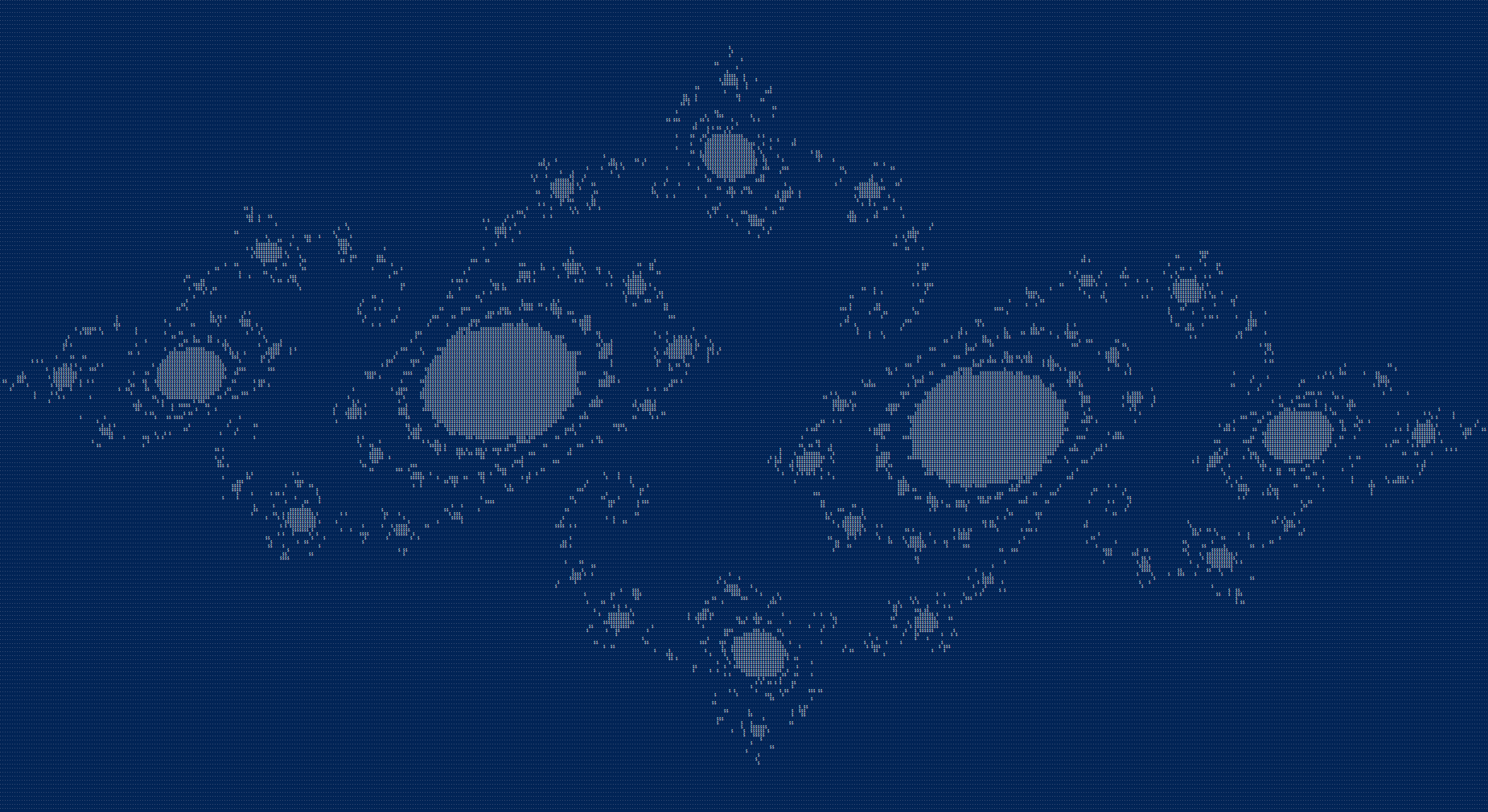
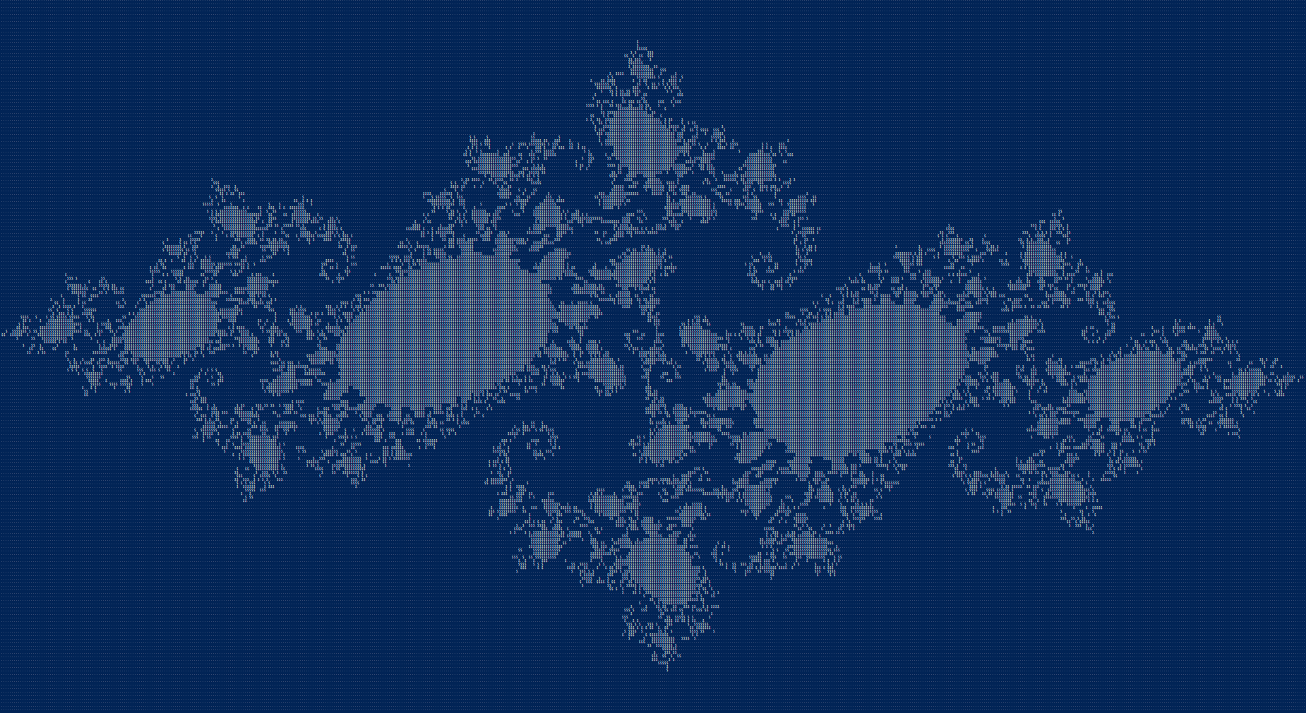
These next images show what my program outputs for \(c = -0.75 + 0.11i\) and \(c = -0.74543 + 0.11301i\text{,}\) respectively. One thing I'll note is that for especially skinny Julia sets, such as the one for \(c = -0.8i\text{,}\) the program barely draws anything.
If you want to compare these drawings to more professional and detailed renders, check the Wikipedia page on Julia sets, and scroll down a bit to see the images. Or just read the whole article, while you're there. You'll also find some pseudocode which implements much the same process I outlined above.
That's all for today. Julia sets—kinda neat.